H

The hand pump is a positive displacement pump which, because of its small size, can be held in the hand and actuated manually such as a lever pump or a hand piston pump.

HART stands for "Highway Addressable Remote Transducer" and is a standardised communication protocol for industrial field buses. It enables communication among multiple participants via a common data bus and is based on the 4/20 mA standard used to transmit analog sensor signals (also see Communications system).

This term is an important energy concept (DIN EN ISO 17769-1) in centrifugal pump engineering. A distinction must be made between the pump head and the system head.

The pump head is the hydraulic power or pump output power (P_Q) transmitted to the fluid handled relative to ρ · g · Q. 

The sum of all power (positive input, negative output) represented by the pump power output (P_Q) must be zero within the boundaries of the system. See Fig. 1 Head

If the expression P_Q.d – P_Q.s represents the pump power output (P_Q), the useful power output is as follows:

According to BERNOULLI (see Fluid mechanics) the equation for useful power output is:

For the pump head, this means:

If the fluid handled is compressible, the value for density (ρ) should be defined as the arithmetic mean of the density at the pump discharge nozzle and the density at the pump suction nozzle:

The system head can be established in a similar manner, taking into account the head losses (H_L):

The term geodetic head (H_geo) is sometimes used to designate the system head. It refers to the difference in elevation, or height, between the system's outlet cross-section (A_a) and the system's inlet cross-section (A_e):

Under steady-state conditions (rotational speed (n) = constant), the pump head is equal to the system head.

The unit of head is metres (m). The following expressions are also used in conjunction with the term head.

Heads and their significance

• Head at BEP (H_opt): pump head at the best efficiency point
• Nominal head (H_N): pump head for which the pump has been designed
• Upper head limit (H_max): max. permissible head at which the pump can be continuously operated without suffering damage
• Lower head limit (H_min): min. permissible head at which the pump can be operated without suffering damage
• Shut-off head (H₀): head for a flow rate Q = 0 m³/s
• Peak head (H_peak): head at apex (relative maximum) of an unstable H/Q curve, see Fig. 4 Characteristic curve
• Static head (H_A,0 or H_stat): the portion of the system head (see System characteristic curve and Characteristic curve) which is independent of the flow rate (Q)
• 

The head coefficient (ψ) is a characteristic coefficient, derived from the corresponding physical quantity according to the affinity laws and used to characterise the operating behaviour. It characterises the head (H) of the pump:

When the head varies at constant rotational pump speed, ψ ~ H. The head coefficient (ψ) is therefore indicative of the ordinate (analogous to H) on H/Q curves plotted in a non-dimensional representation. In conjunction with the specific energy (Y) this results in: 

Head losses are a result of wall friction in all types of pipelines and of local resistance to flow, for example in valves and fittings (see also Pressure loss). 

Recommended flow velocities 

• For cold water:
  Suction line 0.7-1.5 m/s
  Discharge line 1.0-2.0 m/s
• For hot water:
  Suction line 0.5-1.0 m/s
  Discharge line 1.5-3.5 m/s

Head loss in a pipe

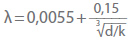
The equation for the head loss of a flow in a straight length of piping with circular cross-section is:

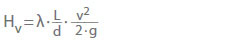
λ   Pipe friction factor
L   Pipe length in m
d   Pipe inside diameter in m 
v   Flow velocity in a cross-section in m/s
     (= 4 Q / π d² with Q in m³/s)
g   Acceleration due to gravity in m/s²

see Fig. 1 and 4. Head loss

The pipe friction factor was established experimentally. It is only dependent on the state of flow of the fluid handled and of the relative roughness (d/k) of the pipes through which the fluid is flowing. For non-circular pipe cross-sections the equivalent diameter in fluid-mechanical terms (d) applies:

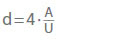
A     Cross-section in m²
U    Wetted cross-section circumference in m
      (the free surface of an open channel is not considered)

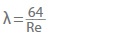
The state of flow is determined by the Reynolds number (Re) according to the affinity laws. The following applies to circular pipes:

v    Flow velocity in a cross-section in m/s
      (= 4 Q / π d2 with Q in m³/s)
ν   Kinematic viscosity in m²/s
     (for water at 20 °C: 1.00 · 10 - 6 m²/s)
d   Pipe inside diameter in m

See Fig. 4 Head loss

For hydraulically smooth pipes such as smooth drawn metal or plastic piping (e. g. PE or PVC), or in the case of laminar flow, the pipe friction factor (λ) can be calculated. For laminar flow in a pipe with a Reynolds number smaller than 2320 the pipe friction factor is independent of roughness:

If flow is turbulent, or the Reynolds number higher than 2320, the pipe friction factor in hydraulically smooth pipes can be represented by an empirical equation according to Eck (due to the fact that deviations are below 1 % if the Reynolds number is lower than 10⁸).

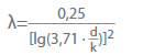
The pipe friction factor (λ) also depends on a further dimensionless parameter, i.e. on the relative roughness of the pipe's inner surface (d/k). Both must be specified in the same unit (e. g. mm).

See Fig. 1 Head loss

(k) is the mean absolute roughness of the pipe inner surface for which approximate values are available depending on the material and manufacturing processes. See Fig. 2 Head loss

Above the limit curve, the pipe friction factor (λ) is solely dependent on the pipe's relative roughness (d/k). See Fig. 1 Head loss

The following empirical equation by Moody can be used for this region:

For practical use, the head loss (HL) per 100 m of straight steel pipe is shown in the diagram as a function of the flow rate (Q) and pipe inside diameter (d).
See Fig. 3 Head loss

The values are valid only for cold, clean water or for fluids with the same kinematic viscosity, for completely filled pipes and for absolute roughness of the pipe inner surface of k = 0.05 mm.

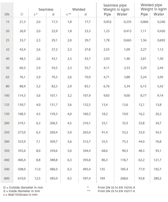
Dimensions, weights, water fill for new seamless or longitudinally welded steel pipes
See  Fig. 4 Head loss

The effect of an increased surface roughness k will be demonstrated in the following for a frequently used set of parameter ranges (nominal diameter DN = 50 to 300, flow velocity v = 0.8 to 3.0 m/s). See Fig. 3 Head loss

The light blue region corresponds to the similarly marked region for an absolute mean roughness of k = 0.05 mm.
See Fig. 1 Head loss

For a roughness increased by a factor of 6 (slightly incrusted old steel pipe with k = 0.30 = 300 μm (0.30 mm), the pipe friction factors (and the associated proportional head losses) in the dark blue region are only 25 - 60 % higher than before.
See Fig. 1 Head loss

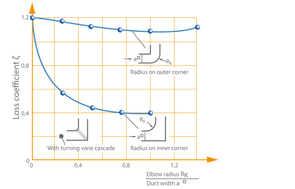
Loss coefficients ζ for pipe bends and elbows
See Fig. 8 Head loss

For sewage pipes the increased roughness caused by soiling must be taken into consideration. For pipes subject to extreme incrustation, the actual head loss can only be determined experimentally. Deviations from the nominal diameter change the head loss considerably, as the pipe inside diameter features in the equation to the 5th power.

A 5 % reduction of the inside diameter, for example, leads to an increase in head loss by as much as 30 %.  It is therefore important that the internal diameter is not simply replaced with the nominal diameter in the calculations.

The head losses in plastic pipes or smooth drawn metal piping are very low thanks to the smooth pipe surfaces. The head losses established are valid for water at 10 °C. At other temperatures, the loss for plastic pipes must be multiplied by a specified temperature correction factor to account for their larger thermal expansion. For sewage or other untreated water, an additional 20-30 % head loss should be taken into account for potential deposits.

Head losses for plastic and smooth drawn metal pipes

See Fig. 5 Head loss

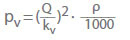
Head losses in valves and fittings

The head loss (H_L) in valves and fittings is given by:

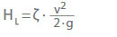
See Figs. 6 to 12 Head loss

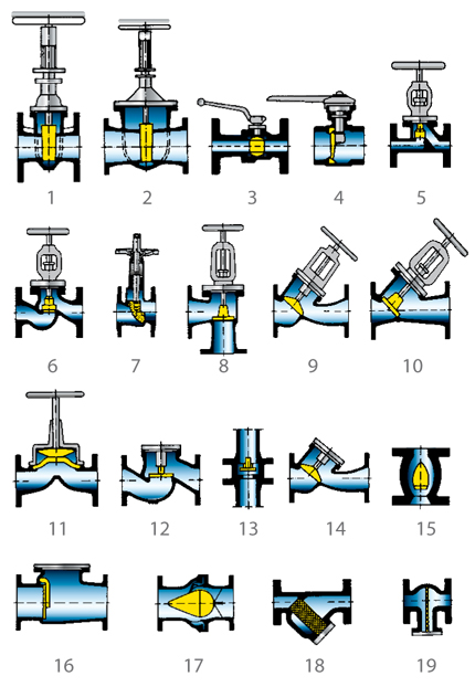
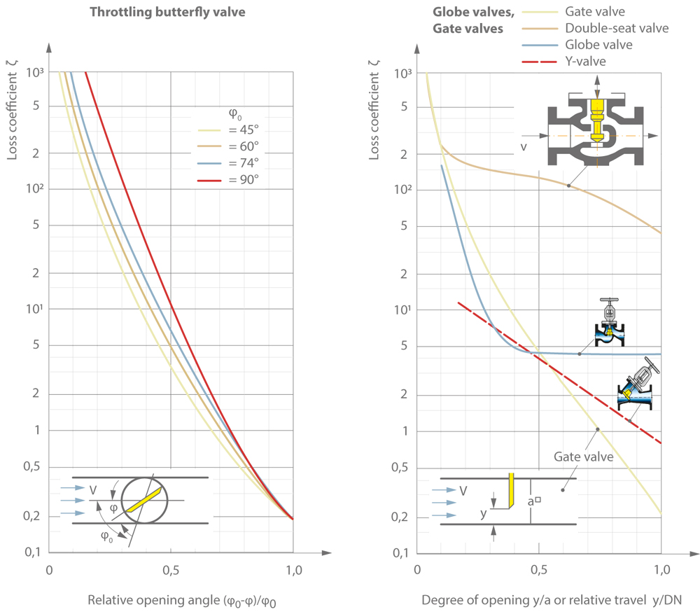
The losses attributable to the straightening of the flow disturbances over a pipe length equivalent to 12 x DN downstream of the valve are included in the loss coefficients in accordance with the VDI/VDE 2173 guideline. The values apply to valves which have a steady approach flow, are fully opened and operated with cold water. Depending on the inlet and outlet flow conditions, the valve models and development objectives (i. e. inexpensive or energy-saving valves), the loss values can vary dramatically.

See Fig. 7 Head loss

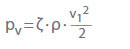
Often the k_v value is used instead of the loss coefficient (ζ) when calculating the pressure loss for water in valves:

The k_v value is the flow rate in m³/h which would result from a pressure drop p_v = 1 bar through the valve for cold water. It describes the correlation between the pressure loss (p_L) in bar and the flow rate (Q) in m³/h. Conversion to flow coefficient ζ for cold water:

d   Reference (nominal) diameter of the valve in cm

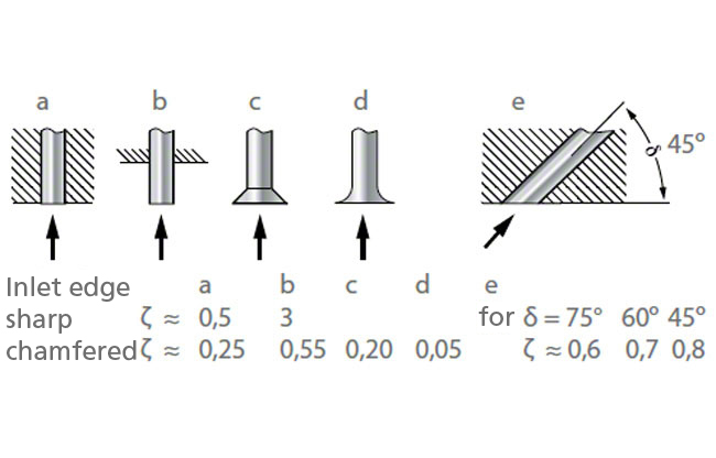
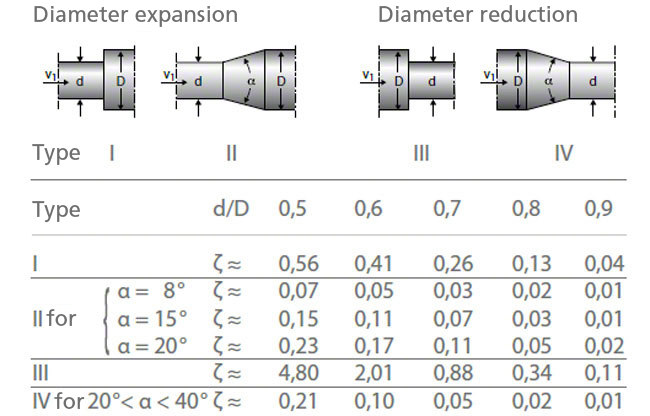
For the calculation of head losses in fittings, branch fittings and adapters require a different approach. See Figs. 9 and 10 Head loss

For all fittings a differentiation must be made between two forms of pressure loss:

• Irreversible pressure losses (reduction in pressure)

• Reversible pressure changes of the frictionless flow according to Bernoulli's equation

For accelerated flows such as reductions in the pipe diameter, (p₂ − p₁) is always negative; for decelerated flows such as pipe expansions, it is always positive. When calculating the net pressure change as the arithmetic sum of pL and (p₂ − p₁), the irreversible pressure losses must always be subtracted.

Influence of highly viscous fluids on the system characteristic curve

As the laws of fluid dynamics retain their validity for all Newtonian fluids, the equations and diagrams for calculating the pipe friction factors and loss coefficients for valves are also applicable to viscous fluids with a higher viscosity than water.

When calculating the Reynolds number Re = v · d / ν , one must simply substitute the kinematic viscosity of the viscous fluids ν_z for the water viscosity ν_z.

This yields a lower Re number and, according to Fig. 1 Head loss, a larger pipe friction coefficient λ_z (Note: the influence of the wall roughness can now often be ignored because of the larger boundary layer thickness in the flow).
All of the pressure losses in the pipes and valves calculated for water are to be extrapolated using the ratio λ_z/λ_w.

Figure 13 Head loss is also suitable for general practical use.

The pipe friction factor λ_z can be determined quickly as a function of the flow rate Q, pipe inside diameter d and kinematic viscosity ν_z. It must be kept in mind, however, that the coefficient λ_w in this diagram is only valid for hydraulically smooth pipes (i.e. not for rough pipes)! The corresponding λ_w can be used to calculate the ratio λ_z/λ_w.

As the static component of the system characteristic curve Hsys , see Fig. 1 System characteristic curve and Fig. 2 Head, is not affected by viscosity, the dynamic component of the system characteristic curve for water can be redrawn as a steeper parabola for a viscous fluid.

Influence of non-Newtonian fluids on the system characteristic curve

As the flow curves are not straight lines of constant linear viscosity, the calculation of the head losses is very cumbersome. In this case, loss calculation is based on experience with particular fluids.

Heat is another term for heat energy.

The heat barrier helps prevent the heat transferring from the hot pump to the cold motor so that the insulation of the stator winding (see Asynchronous motor), which has a limited temperature resistance, is not compromised. It is fitted between the pump and motor of glandless circulating pumps. A heat barrier can be cooled with water but in order to keep cooling water demands and energy losses as low as possible it is better to reduce the heat transfer. It is therefore important when designing the pump that the cross-sections which transfer the heat are built as small as possible by incorporating air pockets, and that materials of low thermal conductivity are used.
See Fig. 1 Heat barrier

The heat barrier must be able to resist mechanical strain as the tie bolts clamp the heat barrier between the motor housing and the pump casing.

Heat energy in the technical sense means the thermal energy, that a body possesses. The  SI unit is the J (Joule).

1 J = 1 Nm = 1 Ws or 1 kcal = 4.1868 kJ

The heat pump is not a pump in the strict sense of the word, but a system with the aid of which low temperature heat can be elevated ("pumped up") to a higher temperature level. The heat pump operates on the thermodynamic principle of a refrigeration system. It allows the exploitation of the energy provided by heat sources such as air, water and soil, and also the exploitation of waste heat from industrial processes.

A heat pump system usually comprises two heat exchangers (liquefier and evaporator), an expansion valve and a compressor. The circuit is primed with a liquid refrigerant which evaporates at low temperature and absorbs heat from its surroundings. The compressor then raises the refrigerant to a higher pressure and temperature level, after which it is fed through the liquefier, where it condenses. The heat released during condensation is transmitted to a heating circuit (see Circulator pump) In the final stage the liquid refrigerant is expanded in the expansion valve and the cycle starts anew. See Fig. 1 Heat pump

The supply temperature which is capable of being attained economically in hot water heating systems or service water supply systems can amount to up to 55 °C. Heat pump systems have so far been installed mainly for room heating, service water heating and swimming pool water heating purposes, usually in conjunction with conventional heating systems (as bivalent heating system).

A heat transfer pump is a pump used for circulating heat transfer fluids, e.g. for maintaining the heat transfer fluid circulation in a heating system. 

Since the temperature of thermal oils can reach up to 350 °C, a cooling section (usually with air) must be used between the pump casing and the shaft seal to reduce high temperatures so that normal product-lubricated plain bearings (e.g. carbon bush) and standard mechanical seals can be employed. See Fig. 1 Heat transfer pump

High specific speed is a parameter used to characterise turbomachinery speed.

A high-efficiency motor operates at a high level of efficiency and is compliant with efficiency class IE3 or IE4 at minimum.

The high-pressure pump is a centrifugal pump with a head of between 200 and 1200 m, which is used, for example, in pressure booster systems, Low-pressure, medium-pressure or super-pressure pumps are used for other areas of application.

High-speed centrifugal pumps are geared pumps used, for example, to remove sandy soil from an open-cast mine. 
See Fig. 1 Geared pump

HMI stands for "Human-Machine Interface" and is also referred to as the "Man-Machine Interface" (MMI). It is used to operate, monitor, and control processes in an MMI system. Required information is provided to the operator in analog form via signal lamps, display panels, and buttons, or digitally via a visualisationsystem, by way of a terminal (see Communications system).

Horizontal pumps are centrifugal pumps with horizontal shaft axis.

The hot water pump is a centrifugal pump for handling water at temperatures above 100 ºC. They are used for boiler feeding (see Boiler feed pump), central heating (see Circulator pump) and feed water circulation, and also as circulating pumps in nuclear plants (see Reactor pump). 

Materials frequently used for hot water pumps are cast iron, nodular cast iron, cast steel, cast chrome steel and austenitic cast steel as well as appropriate wrought alloys for specific pump casings. 

In the event of sudden temperature changes, considerable stresses act in the tie bolts of ring-section pumps and in the barrels of barrel pull-out pumps.

In order to prevent any shifting of the pump and motor shaft centrelines towards one another under the influence of the high casing temperature, the pump feet are usually arranged at shaft centreline height on the pump casing. This pump foot arrangement is characteristic of hot water pumps in ring-section design. 

See Fig. 1 Hot water pump

In single-stage hot water pumps, the feet are very often also arranged at the bottom of the pump casing. 

See Fig. 2 Hot water pump

To compensate for unavoidable shaft displacement, double Cardan couplings are used (see Shaft coupling). These offer a reliable alternative to pump casings with feet at the centreline.

Depending on temperature and pressure conditions, the casing is sealed (see Sealing element) by O-rings, spiral-wound gaskets or flat gaskets. 

The shaft seal must operate at a low temperature level. For this reason, frictional heat is dissipated. This is done either by means of an external coolant which supplies the shaft seal chamber or heat exchanger, or may alternatively be effected by environmentally friendly air cooling.

See Fig. 2 Hot water pump

Mechanical seals or occasionally even gland packings or floating ring seals can be used as types of seal (see Shaft seal). 

The shaft itself runs in oil-lubricated rolling element or plain bearings cooled by air, oil or water.

On tubular casing pumps, particularly those of an axial flow type, the flow velocity downstream of the impeller can be reduced by means of a hub diffuser. The free flow cross-section is enlarged by a gradual reduction of the hub diameter.
Hub diffusers are subject to the risk of flow separation both at the inner hub contour and at the cylindrical outer contour (see Flow separation).

The hub-to-tip ratio (ν) represents a characteristic geometric dimension of centrifugal pumps' impellers and is usually defined as follows:

The choice of hub-to-tip ratio should ensure optimal suction characteristics. The efficiency at various specific speeds and design aspects such as adjustable blades for waste water handling are some of the significant factors determining the best possible choice of hub-to-tip ratio.

Hybrid cooling is a form of cooling which combines the benefits of dry and wet cooling at markedly reduced water consumption. The benefits are high-level cooling capacity and improved efficiency. As water is evaporated in this cooling process, it is assigned to wet cooling.
Alternative cooling processes are wet or dry cooling.

Hydraulic efficiency (η_h) is also referred to as "vane efficiency" in the specialist centrifugal pump engineering literature and is the quotient of pump power output (P_Q) and vane power (P_vane).

P                     Power input of a centrifugal pump
P_Lm/Ldiscfric        Mechanical power loss in plain bearings and rolling element bearings, shaft                           seals and in the impeller side gaps (see Disc friction)

Hydraulic rams, or hydrams, are relatively simple machines, with the help of which water can be lifted to a higher geodetic level or pressure level.

The kinetic energy contained in flowing water, retained by sudden closing of a valve, generates surge pressure strong enough to force part of the water into an accumulator (air vessel). The delivery pipe (riser) is fed from here.
See Fig. 1 Hydraulic ram

After opening the valve, the water column is once again placed in motion under the influence of a slight drop, so that the process continually repeats.

This type of transport, though transient, uses no outside energy and, apart from occasional inspections of the two valves (i.e. the only moving parts), is maintenance-free. The hydraulic ram is therefore particularly suitable for irrigation purposes in developing countries.

Hydraulic torque converters resemble fluid couplings and consist of an impeller (on the input shaft), runner (on the output shaft) and a vaned diffuser which absorbs torque (T_Le) and is supported by the casing. There is a balancing of moments between the input torque (T_P) (impeller torque), the output torque (T_T) (runner torque) and the torque at the vaned diffuser (T_Le).

Given that the hydraulic torque converter is responsible for converting the impeller torque into runner torque, it is also referred to as a torque converter. Within the context of drivingcentrifugal pumps, these components only play a secondary role, except in the case of pumped storage power plants.

Hydraulic unbalance during pump operation has the same effects as mechanical unbalance.

A hydrodynamic coupling is a type of fluid coupling used to transmit  torque.

A hydrodynamic transmission is a hydraulic torque converter, that sets a fluid in motion internally in order to drive an output element.